Radar calibration sphere flight: 2 December 2010: Difference between revisions
No edit summary |
(Updated to use math mode, added categories) |
||
| Line 3: | Line 3: | ||
==Introduction== | ==Introduction== | ||
The preferred sphere | The preferred sphere calibration method used at CHILL is the free-flying sphere. A 12 inch diameter Styrofoam sphere is wrapped with aluminum foil and suspended below a 600 gram helium filled balloon. The balloon is then released and tracked optically, at first, with a theodolite. Once the sphere has traveled 5 or so kilometers downwind of the radar, its position is relayed to the radar operator, who sets a tight sector scan to cover the sphere's position. | ||
The main advantage of the free-flying sphere calibration is that the sphere is carried up to elevation angles which are well above any interference from ground targets, which are often a problem with tethered sphere calibrations. | The main advantage of the free-flying sphere calibration is that the sphere is carried up to elevation angles which are well above any interference from ground targets, which are often a problem with tethered sphere calibrations. | ||
It is important to | It is important to set up the radar for over-sampling of the sphere. The CHILL radar pulse length can be set to one microsecond, while the receiver sample spacing can be set to 30 meters or 0.2 microseconds. This ensures that there will always be a receiver sample situated at a range which is optimal for capturing the peak return from the sphere. The sector scans are also adjusted to over-sample in azimuth and elevation. Specifically, they are set to provide 0.1 degree sample spacing in both azimuth and elevation. Given the one degree antenna beamwidth, this ensures that each volume scan should have many samples which intersect the sphere, and that several of these will have the center of the sphere at or very close the boresite of the antenna. | ||
==Gain Calibration== | |||
In processing the data, each ray of data is filtered by several constraints such as, beyond a minimum range, above a specified signal to noise ratio, and non-zero velocity. Those samples that pass these tests are converted to an equivalent antenna gain using the point target radar equation: | |||
<center> | <center> | ||
< | <math> | ||
G = \sqrt{\frac{64 P_r \pi^3 R^4}{P_t \sigma \lambda^2}} | |||
</math> | |||
</ | |||
</center> | </center> | ||
Where: | |||
<center> | |||
{| {{Prettytable}} | |||
!{{Hl3}} | Variable | |||
{| | !{{Hl3}} | Meaning | ||
|G | |- | ||
|<math>G</math> | |||
|Antenna Gain - Waveguide Losses | |Antenna Gain - Waveguide Losses | ||
|- | |- | ||
| | |<math>P_r</math> | ||
|Received Power | |Received Power | ||
|- | |- | ||
|R | |<math>R</math> | ||
|Range to sample | |Range to sample | ||
|- | |- | ||
| | |<math>P_t</math> | ||
|Transmitted Power | |Transmitted Power | ||
|- | |- | ||
|sigma | |<math>\sigma</math> | ||
|Crossection area of sphere | |Crossection area of sphere | ||
|- | |- | ||
|lambda | |<math>\lambda</math> | ||
|Radar wavelength | |Radar wavelength | ||
|} | |} | ||
</center> | |||
For each ray, the peak gain and the range at which it occurred is saved in a file. This file is read by a Perl script which generates a histogram of all the observed gain points. When the histogram is plotted, one can see the towards the right hand side of the plot a fairly sharp drop off in frequency of occurrence. This drop-off is located at the location of the peak observed gain. i.e. The point where those few measurements where the antenna was pointed directly at the sphere. In the plot below, the arrow is drawn at the gain from a solar calibration run on about the same date. | For each ray, the peak gain and the range at which it occurred is saved in a file. This file is read by a Perl script which generates a histogram of all the observed gain points. When the histogram is plotted, one can see the towards the right hand side of the plot a fairly sharp drop off in frequency of occurrence. This drop-off is located at the location of the peak observed gain. i.e. The point where those few measurements where the antenna was pointed directly at the sphere. In the plot below, the arrow is drawn at the gain from a solar calibration run on about the same date. | ||
[[Image:Sphcal02dec2010.png]] | [[Image:Sphcal02dec2010.png]] | ||
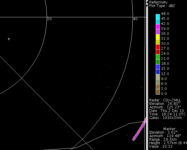
==Reflectivity loop== | |||
<center> | |||
<imgloop delay=200 imgprefix="http://www.chill.colostate.edu/anim/2dec2010_sphere/" width=640 height=512> | |||
dBZ.CHL20101202_182341 sphere_os PPI Sweep 03 Plot 0.png | |||
dBZ.CHL20101202_182455 sphere_os PPI Sweep 04 Plot 0.png | |||
dBZ.CHL20101202_182544 sphere_os PPI Sweep 12 Plot 0.png | |||
dBZ.CHL20101202_182933 sphere_os PPI Sweep 02 Plot 0.png | |||
dBZ.CHL20101202_183027 sphere_os PPI Sweep 04 Plot 0.png | |||
dBZ.CHL20101202_183217 sphere_os PPI Sweep 05 Plot 0.png | |||
dBZ.CHL20101202_183421 sphere_os PPI Sweep 02 Plot 0.png | |||
dBZ.CHL20101202_183612 sphere_os PPI Sweep 01 Plot 0.png | |||
dBZ.CHL20101202_183744 sphere_os PPI Sweep 02 Plot 0.png | |||
</imgloop> | |||
</center> | |||
[[Category:Featured Articles]] | |||
[[Category:Calibration]] | |||
[[Category:Sphere Calibration]] | |||
Revision as of 12:19, 1 January 2011
Overview
On December 2nd 2010 a sphere calibration was conducted at the radar. Sphere calibrations are fairly unique in that they test the entire radar, both transmitter and receiver. The provide a measurement of the (antenna gain - waveguide loss). This measurement is required to calculate absolute reflectivity. The sphere calibration should agree with and lend support to comparable measurements provided by solar or standard gain horn calibrations.
Introduction
The preferred sphere calibration method used at CHILL is the free-flying sphere. A 12 inch diameter Styrofoam sphere is wrapped with aluminum foil and suspended below a 600 gram helium filled balloon. The balloon is then released and tracked optically, at first, with a theodolite. Once the sphere has traveled 5 or so kilometers downwind of the radar, its position is relayed to the radar operator, who sets a tight sector scan to cover the sphere's position.
The main advantage of the free-flying sphere calibration is that the sphere is carried up to elevation angles which are well above any interference from ground targets, which are often a problem with tethered sphere calibrations.
It is important to set up the radar for over-sampling of the sphere. The CHILL radar pulse length can be set to one microsecond, while the receiver sample spacing can be set to 30 meters or 0.2 microseconds. This ensures that there will always be a receiver sample situated at a range which is optimal for capturing the peak return from the sphere. The sector scans are also adjusted to over-sample in azimuth and elevation. Specifically, they are set to provide 0.1 degree sample spacing in both azimuth and elevation. Given the one degree antenna beamwidth, this ensures that each volume scan should have many samples which intersect the sphere, and that several of these will have the center of the sphere at or very close the boresite of the antenna.
Gain Calibration
In processing the data, each ray of data is filtered by several constraints such as, beyond a minimum range, above a specified signal to noise ratio, and non-zero velocity. Those samples that pass these tests are converted to an equivalent antenna gain using the point target radar equation:

Where:
| Variable | Meaning |
|---|---|
| Antenna Gain - Waveguide Losses | |
| Received Power | |
| Range to sample | |
| Transmitted Power | |
| Crossection area of sphere | |
| Radar wavelength |


For each ray, the peak gain and the range at which it occurred is saved in a file. This file is read by a Perl script which generates a histogram of all the observed gain points. When the histogram is plotted, one can see the towards the right hand side of the plot a fairly sharp drop off in frequency of occurrence. This drop-off is located at the location of the peak observed gain. i.e. The point where those few measurements where the antenna was pointed directly at the sphere. In the plot below, the arrow is drawn at the gain from a solar calibration run on about the same date.

Reflectivity loop
|
|
||
|