DPWX/Modeling observed drop size distributions: 23 May 2015: Difference between revisions
Pat kennedy (talk | contribs) (initial fixed image posting) |
m (Jgeorge moved page DPWX/Modeling observed drop size distributions: 23 May 2015. to DPWX/Modeling observed drop size distributions: 23 May 2015) |
||
| (14 intermediate revisions by one other user not shown) | |||
| Line 1: | Line 1: | ||
Authors: Merhala Thurai, Patrick C. Kennedy, and V. N. Bringi | |||
[[Image:MPS and SN36 23May 2015 2042 450w inset 2.png|300px|right]] | |||
Drop size distribution (DSD) derived from the combined measurements from two optical disdrometers (an MPS and a 2DVD) installed at the Easton Airport (13 km SSE of CSU-CHILL). This rainfall was associated with ~50 dBZ reflectivity at Easton (PPI inset plot). The red dashed line is a generalized gamma distribution fit to the composite DSD data. Three minute DSDs, their fits, and the CSU-CHILL dual-polarization data from various rain rates measured at Easton on 23 May 2015 have been prepared. | |||
==Introduction== | |||
From April 2015, a six-month rain measurement campaign was initiated at the Easton site 13 km SSE from the CHILL radar site. The campaign involved (i) a 2-D video disdrometer [2DVD, Shönhuber et al., 2008], (ii) a droplet spectrometer called the meteorological particle spectrometer [MPS, Baumgardner et al., 2002], (iii) a Pluvio raingauge [OTT Messtechnik GmbH, 2010], and (iv) a precipitation occurrence sensor system [POSS, Sheppard and Joe, 2008]) all installed within a 2/3rd scaled DFIR double wind fence that was originally installed for the MASCRAD snow observation project '''[[ DPWX/Initial Multiple Angle Snow Camera-Radar experiment (MASCRAD) project operations: 15 November 2014|(earlier article here.)]]'''. Many events were recorded by the ground instruments, and for several of these events, a near-complete picture of the rain drop size spectra (from very small to large drops) were derived, by combining the MPS measurements for small drops (< 1 mm) and the 2DVD measurements for larger drops. The shapes of the combined drop size distribution (DSD) spectra had pointed to the need for more flexible model to represent the full DSD [Thurai et al., 2017; Thurai and Bringi, 2017] rather than the standard gamma model. Here we consider a formulation based on the generalized gamma model, previously considered in [Lee et al., 2004 and Raupach and Berne, 2017] for rain DSDs. Specifically, equation (43) in [Lee et al., 2004] is used to derive/fit the four parameters governing this equation, and by setting i=3 and j=4, i.e. using the third and the fourth moments. Here we show a selected case event that occurred on 23 May 2015 which lasted for 90 minutes over Easton, resulting in a total event accumulation of 15 mm. Large drops were recorded by the 2DVD. One example is given below (constructed from the 2DVD front and side view contours, after correcting for any image distortions arising from drop horizontal velocity). | |||
[[Image:Drop image 640w.png|center]] | [[Image:Drop image 640w.png|center]] | ||
A summary of the DSD measurements from the 2DVD are shown below. Around 20:45 UTC, wide DSD spectra can be seen with drop diameters ranging up to 5 mm and higher. | |||
[[Image:DSD time series w640.png|center]] | |||
==Reflectivity loop== | |||
The following loop shows the CSU-CHILL S-band reflectivity data collected in a series of 1.5 degree elevation angle 360 degree surveillance scans that were repeated at ~90 second intervals during the 2028 - 2218 UTC period. This is the lowest elevation angle that is free of ground clutter in the immediate vicinity of the Easton instrumentation site. A wide range of reflectivity values occurred at Easton (marked with a '+ E' sign as various echoes crossed the site in the southerly synoptic flow regime. Maximum reflectivities of ~50 dBZ occurred around the time (2045) when the ~5 mm diameter drop was observed in the first plot shown above. | |||
<center> | |||
<imgloop delay=200 imgprefix="http://www.chill.colostate.edu/anim/MT_oct_2017_23may2015_easton/" width=640 height=512> | |||
dBZ.CHL20150523_202819 GFC_1 PPI Sweep 01 Plot 0.png | |||
dBZ.CHL20150523_202951 GFC_1 PPI Sweep 01 Plot 0.png | |||
dBZ.CHL20150523_203122 GFC_1 PPI Sweep 01 Plot 0.png | |||
dBZ.CHL20150523_203254 GFC_1 PPI Sweep 01 Plot 0.png | |||
dBZ.CHL20150523_203425 GFC_1 PPI Sweep 01 Plot 0.png | |||
dBZ.CHL20150523_203557 GFC_1 PPI Sweep 01 Plot 0.png | |||
dBZ.CHL20150523_203729 GFC_1 PPI Sweep 01 Plot 0.png | |||
dBZ.CHL20150523_203900 GFC_1 PPI Sweep 01 Plot 0.png | |||
dBZ.CHL20150523_204032 GFC_1 PPI Sweep 01 Plot 0.png | |||
dBZ.CHL20150523_204204 GFC_1 PPI Sweep 01 Plot 0.png | |||
dBZ.CHL20150523_204335 GFC_1 PPI Sweep 01 Plot 0.png | |||
dBZ.CHL20150523_204507 GFC_1 PPI Sweep 01 Plot 0.png | |||
dBZ.CHL20150523_204638 GFC_1 PPI Sweep 01 Plot 0.png | |||
dBZ.CHL20150523_204810 GFC_1 PPI Sweep 01 Plot 0.png | |||
dBZ.CHL20150523_204941 GFC_1 PPI Sweep 01 Plot 0.png | |||
dBZ.CHL20150523_205113 GFC_1 PPI Sweep 01 Plot 0.png | |||
dBZ.CHL20150523_205245 GFC_1 PPI Sweep 01 Plot 0.png | |||
dBZ.CHL20150523_205416 GFC_1 PPI Sweep 01 Plot 0.png | |||
dBZ.CHL20150523_205548 GFC_1 PPI Sweep 01 Plot 0.png | |||
dBZ.CHL20150523_205719 GFC_1 PPI Sweep 01 Plot 0.png | |||
dBZ.CHL20150523_205851 GFC_1 PPI Sweep 01 Plot 0.png | |||
dBZ.CHL20150523_210023 GFC_1 PPI Sweep 01 Plot 0.png | |||
dBZ.CHL20150523_210154 GFC_1 PPI Sweep 01 Plot 0.png | |||
dBZ.CHL20150523_210326 GFC_1 PPI Sweep 01 Plot 0.png | |||
dBZ.CHL20150523_210457 GFC_1 PPI Sweep 01 Plot 0.png | |||
dBZ.CHL20150523_210629 GFC_1 PPI Sweep 01 Plot 0.png | |||
dBZ.CHL20150523_210801 GFC_1 PPI Sweep 01 Plot 0.png | |||
dBZ.CHL20150523_210932 GFC_1 PPI Sweep 01 Plot 0.png | |||
dBZ.CHL20150523_211104 GFC_1 PPI Sweep 01 Plot 0.png | |||
dBZ.CHL20150523_211235 GFC_1 PPI Sweep 01 Plot 0.png | |||
dBZ.CHL20150523_211407 GFC_1 PPI Sweep 01 Plot 0.png | |||
dBZ.CHL20150523_211538 GFC_1 PPI Sweep 01 Plot 0.png | |||
dBZ.CHL20150523_211710 GFC_1 PPI Sweep 01 Plot 0.png | |||
dBZ.CHL20150523_211842 GFC_1 PPI Sweep 01 Plot 0.png | |||
dBZ.CHL20150523_212013 GFC_1 PPI Sweep 01 Plot 0.png | |||
dBZ.CHL20150523_212145 GFC_1 PPI Sweep 01 Plot 0.png | |||
dBZ.CHL20150523_212316 GFC_1 PPI Sweep 01 Plot 0.png | |||
dBZ.CHL20150523_212448 GFC_1 PPI Sweep 01 Plot 0.png | |||
dBZ.CHL20150523_212620 GFC_1 PPI Sweep 01 Plot 0.png | |||
dBZ.CHL20150523_212751 GFC_1 PPI Sweep 01 Plot 0.png | |||
dBZ.CHL20150523_212923 GFC_1 PPI Sweep 01 Plot 0.png | |||
dBZ.CHL20150523_213055 GFC_1 PPI Sweep 01 Plot 0.png | |||
dBZ.CHL20150523_213226 GFC_1 PPI Sweep 01 Plot 0.png | |||
dBZ.CHL20150523_213358 GFC_1 PPI Sweep 01 Plot 0.png | |||
dBZ.CHL20150523_213529 GFC_1 PPI Sweep 01 Plot 0.png | |||
dBZ.CHL20150523_213701 GFC_1 PPI Sweep 01 Plot 0.png | |||
dBZ.CHL20150523_213832 GFC_1 PPI Sweep 01 Plot 0.png | |||
dBZ.CHL20150523_214004 GFC_1 PPI Sweep 01 Plot 0.png | |||
dBZ.CHL20150523_214136 GFC_1 PPI Sweep 01 Plot 0.png | |||
dBZ.CHL20150523_214307 GFC_1 PPI Sweep 01 Plot 0.png | |||
dBZ.CHL20150523_214439 GFC_1 PPI Sweep 01 Plot 0.png | |||
dBZ.CHL20150523_214610 GFC_1 PPI Sweep 01 Plot 0.png | |||
dBZ.CHL20150523_214742 GFC_1 PPI Sweep 01 Plot 0.png | |||
dBZ.CHL20150523_214914 GFC_1 PPI Sweep 01 Plot 0.png | |||
dBZ.CHL20150523_215045 GFC_1 PPI Sweep 01 Plot 0.png | |||
dBZ.CHL20150523_215217 GFC_1 PPI Sweep 01 Plot 0.png | |||
dBZ.CHL20150523_215348 GFC_1 PPI Sweep 01 Plot 0.png | |||
dBZ.CHL20150523_215520 GFC_1 PPI Sweep 01 Plot 0.png | |||
dBZ.CHL20150523_215652 GFC_1 PPI Sweep 01 Plot 0.png | |||
dBZ.CHL20150523_215823 GFC_1 PPI Sweep 01 Plot 0.png | |||
dBZ.CHL20150523_215955 GFC_1 PPI Sweep 01 Plot 0.png | |||
dBZ.CHL20150523_220126 GFC_1 PPI Sweep 01 Plot 0.png | |||
dBZ.CHL20150523_220258 GFC_1 PPI Sweep 01 Plot 0.png | |||
dBZ.CHL20150523_220429 GFC_1 PPI Sweep 01 Plot 0.png | |||
dBZ.CHL20150523_221346 GFC_1 PPI Sweep 01 Plot 0.png | |||
dBZ.CHL20150523_221517 GFC_1 PPI Sweep 01 Plot 0.png | |||
dBZ.CHL20150523_221649 GFC_1 PPI Sweep 01 Plot 0.png | |||
dBZ.CHL20150523_221821 GFC_1 PPI Sweep 01 Plot 0.png | |||
</imgloop> | |||
</center> | |||
==Differential reflectivity loop== | |||
The corresponding differential reflectivity (Zdr) values are shown in the next loop. More positive Zdr values, indicative of more oblate drop shapes, generally occurred during the high reflectivity periods. The transitory appearance of negative Zdr values, mainly in the western azimuth sector, is related to rain water draining off of the radome. | |||
<center> | |||
<imgloop delay=200 imgprefix="http://www.chill.colostate.edu/anim/MT_oct_2017_23may2015_easton/ZDR_2/" width=640 height=512> | |||
ZDR.CHL20150523_202819 GFC_1 PPI Sweep 01 Plot 0.png | |||
ZDR.CHL20150523_202951 GFC_1 PPI Sweep 01 Plot 0.png | |||
ZDR.CHL20150523_203122 GFC_1 PPI Sweep 01 Plot 0.png | |||
ZDR.CHL20150523_203254 GFC_1 PPI Sweep 01 Plot 0.png | |||
ZDR.CHL20150523_203425 GFC_1 PPI Sweep 01 Plot 0.png | |||
ZDR.CHL20150523_203557 GFC_1 PPI Sweep 01 Plot 0.png | |||
ZDR.CHL20150523_203729 GFC_1 PPI Sweep 01 Plot 0.png | |||
ZDR.CHL20150523_203900 GFC_1 PPI Sweep 01 Plot 0.png | |||
ZDR.CHL20150523_204032 GFC_1 PPI Sweep 01 Plot 0.png | |||
ZDR.CHL20150523_204204 GFC_1 PPI Sweep 01 Plot 0.png | |||
ZDR.CHL20150523_204335 GFC_1 PPI Sweep 01 Plot 0.png | |||
ZDR.CHL20150523_204507 GFC_1 PPI Sweep 01 Plot 0.png | |||
ZDR.CHL20150523_204638 GFC_1 PPI Sweep 01 Plot 0.png | |||
ZDR.CHL20150523_204810 GFC_1 PPI Sweep 01 Plot 0.png | |||
ZDR.CHL20150523_204941 GFC_1 PPI Sweep 01 Plot 0.png | |||
ZDR.CHL20150523_205113 GFC_1 PPI Sweep 01 Plot 0.png | |||
ZDR.CHL20150523_205245 GFC_1 PPI Sweep 01 Plot 0.png | |||
ZDR.CHL20150523_205416 GFC_1 PPI Sweep 01 Plot 0.png | |||
ZDR.CHL20150523_205548 GFC_1 PPI Sweep 01 Plot 0.png | |||
ZDR.CHL20150523_205719 GFC_1 PPI Sweep 01 Plot 0.png | |||
ZDR.CHL20150523_205851 GFC_1 PPI Sweep 01 Plot 0.png | |||
ZDR.CHL20150523_210023 GFC_1 PPI Sweep 01 Plot 0.png | |||
ZDR.CHL20150523_210154 GFC_1 PPI Sweep 01 Plot 0.png | |||
ZDR.CHL20150523_210326 GFC_1 PPI Sweep 01 Plot 0.png | |||
ZDR.CHL20150523_210457 GFC_1 PPI Sweep 01 Plot 0.png | |||
ZDR.CHL20150523_210629 GFC_1 PPI Sweep 01 Plot 0.png | |||
ZDR.CHL20150523_210801 GFC_1 PPI Sweep 01 Plot 0.png | |||
ZDR.CHL20150523_210932 GFC_1 PPI Sweep 01 Plot 0.png | |||
ZDR.CHL20150523_211104 GFC_1 PPI Sweep 01 Plot 0.png | |||
ZDR.CHL20150523_211235 GFC_1 PPI Sweep 01 Plot 0.png | |||
ZDR.CHL20150523_211407 GFC_1 PPI Sweep 01 Plot 0.png | |||
ZDR.CHL20150523_211538 GFC_1 PPI Sweep 01 Plot 0.png | |||
ZDR.CHL20150523_211710 GFC_1 PPI Sweep 01 Plot 0.png | |||
ZDR.CHL20150523_211842 GFC_1 PPI Sweep 01 Plot 0.png | |||
ZDR.CHL20150523_212013 GFC_1 PPI Sweep 01 Plot 0.png | |||
ZDR.CHL20150523_212145 GFC_1 PPI Sweep 01 Plot 0.png | |||
ZDR.CHL20150523_212316 GFC_1 PPI Sweep 01 Plot 0.png | |||
ZDR.CHL20150523_212448 GFC_1 PPI Sweep 01 Plot 0.png | |||
ZDR.CHL20150523_212620 GFC_1 PPI Sweep 01 Plot 0.png | |||
ZDR.CHL20150523_212751 GFC_1 PPI Sweep 01 Plot 0.png | |||
ZDR.CHL20150523_212923 GFC_1 PPI Sweep 01 Plot 0.png | |||
ZDR.CHL20150523_213055 GFC_1 PPI Sweep 01 Plot 0.png | |||
ZDR.CHL20150523_213226 GFC_1 PPI Sweep 01 Plot 0.png | |||
ZDR.CHL20150523_213358 GFC_1 PPI Sweep 01 Plot 0.png | |||
ZDR.CHL20150523_213529 GFC_1 PPI Sweep 01 Plot 0.png | |||
ZDR.CHL20150523_213701 GFC_1 PPI Sweep 01 Plot 0.png | |||
ZDR.CHL20150523_213832 GFC_1 PPI Sweep 01 Plot 0.png | |||
ZDR.CHL20150523_214004 GFC_1 PPI Sweep 01 Plot 0.png | |||
ZDR.CHL20150523_214136 GFC_1 PPI Sweep 01 Plot 0.png | |||
ZDR.CHL20150523_214307 GFC_1 PPI Sweep 01 Plot 0.png | |||
ZDR.CHL20150523_214439 GFC_1 PPI Sweep 01 Plot 0.png | |||
ZDR.CHL20150523_214610 GFC_1 PPI Sweep 01 Plot 0.png | |||
ZDR.CHL20150523_214742 GFC_1 PPI Sweep 01 Plot 0.png | |||
ZDR.CHL20150523_214914 GFC_1 PPI Sweep 01 Plot 0.png | |||
ZDR.CHL20150523_215045 GFC_1 PPI Sweep 01 Plot 0.png | |||
ZDR.CHL20150523_215217 GFC_1 PPI Sweep 01 Plot 0.png | |||
ZDR.CHL20150523_215348 GFC_1 PPI Sweep 01 Plot 0.png | |||
ZDR.CHL20150523_215520 GFC_1 PPI Sweep 01 Plot 0.png | |||
ZDR.CHL20150523_215652 GFC_1 PPI Sweep 01 Plot 0.png | |||
ZDR.CHL20150523_215823 GFC_1 PPI Sweep 01 Plot 0.png | |||
ZDR.CHL20150523_215955 GFC_1 PPI Sweep 01 Plot 0.png | |||
ZDR.CHL20150523_220126 GFC_1 PPI Sweep 01 Plot 0.png | |||
ZDR.CHL20150523_220258 GFC_1 PPI Sweep 01 Plot 0.png | |||
ZDR.CHL20150523_220429 GFC_1 PPI Sweep 01 Plot 0.png | |||
ZDR.CHL20150523_221346 GFC_1 PPI Sweep 01 Plot 0.png | |||
ZDR.CHL20150523_221517 GFC_1 PPI Sweep 01 Plot 0.png | |||
ZDR.CHL20150523_221649 GFC_1 PPI Sweep 01 Plot 0.png | |||
ZDR.CHL20150523_221821 GFC_1 PPI Sweep 01 Plot 0.png | |||
</imgloop> | |||
</center> | |||
==Differential propagation phase loop== | |||
The final image loop shows the evolution of the differential propagation phase field. Increased shifts in differential propagation with increasing range indicate the presence of significant concentrations of oblate drops (i.e., heavy rain). The high oblate drop concentrations in these heavy rain areas retard the propagation of H polarized radar pulses relative to the propagation speed of V polarized pulses along the same beam path. An episode of rapid phidp increases over short range intervals occurred near Easton around 2045 UTC. | |||
<center> | |||
<imgloop delay=200 imgprefix="http://www.chill.colostate.edu/anim/MT_oct_2017_23may2015_easton/" width=640 height=512> | |||
PHIDP.CHL20150523_202819 GFC_1 PPI Sweep 01 Plot 0.png | |||
PHIDP.CHL20150523_202951 GFC_1 PPI Sweep 01 Plot 0.png | |||
PHIDP.CHL20150523_203122 GFC_1 PPI Sweep 01 Plot 0.png | |||
PHIDP.CHL20150523_203254 GFC_1 PPI Sweep 01 Plot 0.png | |||
PHIDP.CHL20150523_203425 GFC_1 PPI Sweep 01 Plot 0.png | |||
PHIDP.CHL20150523_203557 GFC_1 PPI Sweep 01 Plot 0.png | |||
PHIDP.CHL20150523_203729 GFC_1 PPI Sweep 01 Plot 0.png | |||
PHIDP.CHL20150523_203900 GFC_1 PPI Sweep 01 Plot 0.png | |||
PHIDP.CHL20150523_204032 GFC_1 PPI Sweep 01 Plot 0.png | |||
PHIDP.CHL20150523_204204 GFC_1 PPI Sweep 01 Plot 0.png | |||
PHIDP.CHL20150523_204335 GFC_1 PPI Sweep 01 Plot 0.png | |||
PHIDP.CHL20150523_204507 GFC_1 PPI Sweep 01 Plot 0.png | |||
PHIDP.CHL20150523_204638 GFC_1 PPI Sweep 01 Plot 0.png | |||
PHIDP.CHL20150523_204810 GFC_1 PPI Sweep 01 Plot 0.png | |||
PHIDP.CHL20150523_204941 GFC_1 PPI Sweep 01 Plot 0.png | |||
PHIDP.CHL20150523_205113 GFC_1 PPI Sweep 01 Plot 0.png | |||
PHIDP.CHL20150523_205245 GFC_1 PPI Sweep 01 Plot 0.png | |||
PHIDP.CHL20150523_205416 GFC_1 PPI Sweep 01 Plot 0.png | |||
PHIDP.CHL20150523_205548 GFC_1 PPI Sweep 01 Plot 0.png | |||
PHIDP.CHL20150523_205719 GFC_1 PPI Sweep 01 Plot 0.png | |||
PHIDP.CHL20150523_205851 GFC_1 PPI Sweep 01 Plot 0.png | |||
PHIDP.CHL20150523_210023 GFC_1 PPI Sweep 01 Plot 0.png | |||
PHIDP.CHL20150523_210154 GFC_1 PPI Sweep 01 Plot 0.png | |||
PHIDP.CHL20150523_210326 GFC_1 PPI Sweep 01 Plot 0.png | |||
PHIDP.CHL20150523_210457 GFC_1 PPI Sweep 01 Plot 0.png | |||
PHIDP.CHL20150523_210629 GFC_1 PPI Sweep 01 Plot 0.png | |||
PHIDP.CHL20150523_210801 GFC_1 PPI Sweep 01 Plot 0.png | |||
PHIDP.CHL20150523_210932 GFC_1 PPI Sweep 01 Plot 0.png | |||
PHIDP.CHL20150523_211104 GFC_1 PPI Sweep 01 Plot 0.png | |||
PHIDP.CHL20150523_211235 GFC_1 PPI Sweep 01 Plot 0.png | |||
PHIDP.CHL20150523_211407 GFC_1 PPI Sweep 01 Plot 0.png | |||
PHIDP.CHL20150523_211538 GFC_1 PPI Sweep 01 Plot 0.png | |||
PHIDP.CHL20150523_211710 GFC_1 PPI Sweep 01 Plot 0.png | |||
PHIDP.CHL20150523_211842 GFC_1 PPI Sweep 01 Plot 0.png | |||
PHIDP.CHL20150523_212013 GFC_1 PPI Sweep 01 Plot 0.png | |||
PHIDP.CHL20150523_212145 GFC_1 PPI Sweep 01 Plot 0.png | |||
PHIDP.CHL20150523_212316 GFC_1 PPI Sweep 01 Plot 0.png | |||
PHIDP.CHL20150523_212448 GFC_1 PPI Sweep 01 Plot 0.png | |||
PHIDP.CHL20150523_212620 GFC_1 PPI Sweep 01 Plot 0.png | |||
PHIDP.CHL20150523_212751 GFC_1 PPI Sweep 01 Plot 0.png | |||
PHIDP.CHL20150523_212923 GFC_1 PPI Sweep 01 Plot 0.png | |||
PHIDP.CHL20150523_213055 GFC_1 PPI Sweep 01 Plot 0.png | |||
PHIDP.CHL20150523_213226 GFC_1 PPI Sweep 01 Plot 0.png | |||
PHIDP.CHL20150523_213358 GFC_1 PPI Sweep 01 Plot 0.png | |||
PHIDP.CHL20150523_213529 GFC_1 PPI Sweep 01 Plot 0.png | |||
PHIDP.CHL20150523_213701 GFC_1 PPI Sweep 01 Plot 0.png | |||
PHIDP.CHL20150523_213832 GFC_1 PPI Sweep 01 Plot 0.png | |||
PHIDP.CHL20150523_214004 GFC_1 PPI Sweep 01 Plot 0.png | |||
PHIDP.CHL20150523_214136 GFC_1 PPI Sweep 01 Plot 0.png | |||
PHIDP.CHL20150523_214307 GFC_1 PPI Sweep 01 Plot 0.png | |||
PHIDP.CHL20150523_214439 GFC_1 PPI Sweep 01 Plot 0.png | |||
PHIDP.CHL20150523_214610 GFC_1 PPI Sweep 01 Plot 0.png | |||
PHIDP.CHL20150523_214742 GFC_1 PPI Sweep 01 Plot 0.png | |||
PHIDP.CHL20150523_214914 GFC_1 PPI Sweep 01 Plot 0.png | |||
PHIDP.CHL20150523_215045 GFC_1 PPI Sweep 01 Plot 0.png | |||
PHIDP.CHL20150523_215217 GFC_1 PPI Sweep 01 Plot 0.png | |||
PHIDP.CHL20150523_215348 GFC_1 PPI Sweep 01 Plot 0.png | |||
PHIDP.CHL20150523_215520 GFC_1 PPI Sweep 01 Plot 0.png | |||
PHIDP.CHL20150523_215652 GFC_1 PPI Sweep 01 Plot 0.png | |||
PHIDP.CHL20150523_215823 GFC_1 PPI Sweep 01 Plot 0.png | |||
PHIDP.CHL20150523_215955 GFC_1 PPI Sweep 01 Plot 0.png | |||
PHIDP.CHL20150523_220126 GFC_1 PPI Sweep 01 Plot 0.png | |||
PHIDP.CHL20150523_220258 GFC_1 PPI Sweep 01 Plot 0.png | |||
PHIDP.CHL20150523_220429 GFC_1 PPI Sweep 01 Plot 0.png | |||
PHIDP.CHL20150523_221346 GFC_1 PPI Sweep 01 Plot 0.png | |||
PHIDP.CHL20150523_221517 GFC_1 PPI Sweep 01 Plot 0.png | |||
PHIDP.CHL20150523_221649 GFC_1 PPI Sweep 01 Plot 0.png | |||
PHIDP.CHL20150523_221821 GFC_1 PPI Sweep 01 Plot 0.png | |||
</imgloop> | |||
</center> | |||
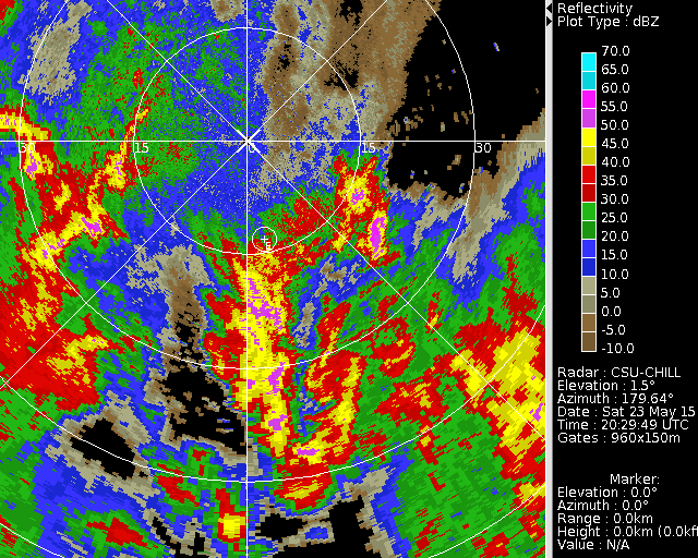
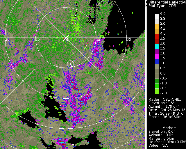
==2045 UTC PPI data== | |||
The three figures below show the low elevation sweep that commenced at 2045:07 UTC. Once again, the location of the ground instrumentation site is marked with a ‘+ E’ sign, i.e. at ~ 13 km range along 171.5 deg azimuth. In this region, high Zh values are seen as well as high Zdr values, indicating the presence of large drops at and around this location around this time period. This is consistent with the DSD data shown earlier. The phidp plot shows significant differential phase shifts beyond the ground instrument site, around 45 deg which is high for S band. | |||
[[Image:DBZ.CHL20150523 204507 GFC 1 PPI Sweep 01 Plot 0.png|center]] | |||
[[Image:ZDR2.ZDR.CHL20150523 204638 GFC 1 PPI Sweep 01 Plot 0.png|center]] | |||
[[Image:DSD | [[Image:PHIDP.CHL20150523 204638 GFC 1 PPI Sweep 01 Plot 0.png|center]] | ||
==DSD data and fits== | |||
The measured DSD spectra (over 3 minutes) which are used as input to the fitting procedure were constructed by utilizing the corresponding MPS-based DSD measurements for 0.15 < Deq ≤ 1 mm and the 2DVD-based DSD measurements for Deq >1 mm. Variation of the data and the fitted curves over the 90-minute period can be seen from the animation below where the MPS data are shown in black, the 2DVD data in blue and the fitted curve in red. In all cases, the fitted curves closely represent the composite DSDs, highlighting the flexibility of the model. | |||
<center> | |||
<imgloop delay=200 imgprefix="http://www.chill.colostate.edu/anim/MT_oct_2017_23may2015_easton/" width=640 height=512> | |||
MPS_and_SN36_23May_2015_Greeley_data_DSD 2021.png | |||
MPS_and_SN36_23May_2015_Greeley_data_DSD 2024.png | |||
MPS_and_SN36_23May_2015_Greeley_data_DSD 2027.png | |||
MPS_and_SN36_23May_2015_Greeley_data_DSD 2030.png | |||
MPS_and_SN36_23May_2015_Greeley_data_DSD 2033.png | |||
MPS_and_SN36_23May_2015_Greeley_data_DSD 2036.png | |||
MPS_and_SN36_23May_2015_Greeley_data_DSD 2039.png | |||
MPS_and_SN36_23May_2015_Greeley_data_DSD 2042.png | |||
MPS_and_SN36_23May_2015_Greeley_data_DSD 2045.png | |||
MPS_and_SN36_23May_2015_Greeley_data_DSD 2048.png | |||
MPS_and_SN36_23May_2015_Greeley_data_DSD 2051.png | |||
MPS_and_SN36_23May_2015_Greeley_data_DSD 2054.png | |||
MPS_and_SN36_23May_2015_Greeley_data_DSD 2057.png | |||
MPS_and_SN36_23May_2015_Greeley_data_DSD 2100.png | |||
MPS_and_SN36_23May_2015_Greeley_data_DSD 2103.png | |||
MPS_and_SN36_23May_2015_Greeley_data_DSD 2106.png | |||
MPS_and_SN36_23May_2015_Greeley_data_DSD 2109.png | |||
MPS_and_SN36_23May_2015_Greeley_data_DSD 2112.png | |||
MPS_and_SN36_23May_2015_Greeley_data_DSD 2115.png | |||
MPS_and_SN36_23May_2015_Greeley_data_DSD 2118.png | |||
MPS_and_SN36_23May_2015_Greeley_data_DSD 2121.png | |||
MPS_and_SN36_23May_2015_Greeley_data_DSD 2124.png | |||
MPS_and_SN36_23May_2015_Greeley_data_DSD 2127.png | |||
MPS_and_SN36_23May_2015_Greeley_data_DSD 2130.png | |||
MPS_and_SN36_23May_2015_Greeley_data_DSD 2133.png | |||
MPS_and_SN36_23May_2015_Greeley_data_DSD 2136.png | |||
MPS_and_SN36_23May_2015_Greeley_data_DSD 2139.png | |||
MPS_and_SN36_23May_2015_Greeley_data_DSD 2142.png | |||
MPS_and_SN36_23May_2015_Greeley_data_DSD 2145.png | |||
MPS_and_SN36_23May_2015_Greeley_data_DSD 2148.png | |||
MPS_and_SN36_23May_2015_Greeley_data_DSD 2151.png | |||
MPS_and_SN36_23May_2015_Greeley_data_DSD 2154.png | |||
MPS_and_SN36_23May_2015_Greeley_data_DSD 2157.png | |||
</imgloop> | |||
</center> | |||
As an independent but qualitative verification of the ‘representativeness’ of the fitted curves, the 3 minute rainfall rates were computed from each of the fitted equations and compared with the 3 minute rain rate measurements from the collocated Pluvio. In the figure below the red line represents the estimates based on the fitted model and the purple line shows the Pluvio measurements. Shown below this plot are two examples of 3-minute DSD measurements and their corresponding fits. The left panel shows the plot for the 20:42 – 20:45 UTC period when the rainfall rate reached its maximum value of 60 mm / h, and by contrast the right panel shows the plot for 21:39 – 21:42 UTC period when the rainfall rate was below 5 mm/h. Once again, the flexibility of the fitted model is clearly evident. The model is able to capture the shape of the DSD curves for a wide range of rainfall rates. Note also that in some cases, the shapes of the DSD's resemble equilibrium DSD curves (e. g. McFarquhar, 2004). | |||
[[Image:Sanity check 640w.png|center]] | |||
[[Image:2042UTC fit.png|center]] | |||
[[Image:2139 fit.png|center]] | |||
==References== | |||
Baumgardner, D., G. Kok, W. Dawson, D. O’Connor, and R. Newton, 2002: A new ground-based precipitation spectrometer: The Meteorological Particle Sensor (MPS). 11th Conf. on Cloud Physics, Ogden, UT, Amer. Meteor. Soc., 8.6. [Available online at https://ams.confex.com/ams/11AR11CP/webprogram/Paper41834.html] | |||
Lee, G., I. Zawadzki, W. Szyrmer, D. Sempere-Torres, and R. Uijlenhoet, 2004: ‘A general approach to double-moment normalization of drop size distributions’, J. Appl. Meteor., 43, 264–281. | |||
McFarquhar, G.M., 2004: A new representation of collision-induced breakup of raindrops and its implications for the shapes of raindrop size distributions. J. Atmos. Sci., 61, 777-794. | |||
OTT Messtechnik GmbH, 2010: “Operating instructions Precipitation Gauge OTT Pluvio”. | |||
Raupach, T.H. and A. Berne, 2017: Invariance of the Double-Moment Normalized Raindrop Size Distribution through 3D Spatial Displacement in Stratiform Rain. J. Appl. Meteor. Climatol., 56, 1663–1680. | |||
Sheppard, B. E., and P. Joe, 2008: Performance of the precipitation occurrence sensor system as a precipitation gauge, Journal of Atmospheric and Oceanic Technology, Vol. 25, pp. 196-212. | |||
Shönhuber, M., G. Lammar and W. L. Randeu, 2008: “The 2D-video-vistrometer”, Chapter 1 in “Precipitation: Advances in Measurement, Estimation and Prediction”, Michaelides, Silas. (Ed.), Springer, ISBN: 978-3-540-77654-3. | |||
Thurai, M. P. Gatlin, V. N. Bringi, W. Petersen, P. Kennedy, B. Notaroš, and L. Carey, 2017: Toward Completing the Raindrop Size Spectrum: Case Studies Involving 2D-Video Disdrometer, Droplet Spectrometer, and Polarimetric Radar Measurements, J. Appl. Meteor. Climatol., 56 (4), 877–896. | |||
Thurai M., and V. N. Bringi, 2017: Application of the Generalized Gamma Model to Represent the Full DSD Spectra, Extended Abstract, 38th Conference on Radar Meteorology, 5A.2, Chicago, USA. https://ams.confex.com/ams/38RADAR/meetingapp.cgi/Paper/320599 | |||
[[ | [[Category:Featured Articles]] | ||
[[Category:Thunderstorm]] | |||
Latest revision as of 18:06, 29 July 2020
Authors: Merhala Thurai, Patrick C. Kennedy, and V. N. Bringi

Drop size distribution (DSD) derived from the combined measurements from two optical disdrometers (an MPS and a 2DVD) installed at the Easton Airport (13 km SSE of CSU-CHILL). This rainfall was associated with ~50 dBZ reflectivity at Easton (PPI inset plot). The red dashed line is a generalized gamma distribution fit to the composite DSD data. Three minute DSDs, their fits, and the CSU-CHILL dual-polarization data from various rain rates measured at Easton on 23 May 2015 have been prepared.
Introduction
From April 2015, a six-month rain measurement campaign was initiated at the Easton site 13 km SSE from the CHILL radar site. The campaign involved (i) a 2-D video disdrometer [2DVD, Shönhuber et al., 2008], (ii) a droplet spectrometer called the meteorological particle spectrometer [MPS, Baumgardner et al., 2002], (iii) a Pluvio raingauge [OTT Messtechnik GmbH, 2010], and (iv) a precipitation occurrence sensor system [POSS, Sheppard and Joe, 2008]) all installed within a 2/3rd scaled DFIR double wind fence that was originally installed for the MASCRAD snow observation project (earlier article here.). Many events were recorded by the ground instruments, and for several of these events, a near-complete picture of the rain drop size spectra (from very small to large drops) were derived, by combining the MPS measurements for small drops (< 1 mm) and the 2DVD measurements for larger drops. The shapes of the combined drop size distribution (DSD) spectra had pointed to the need for more flexible model to represent the full DSD [Thurai et al., 2017; Thurai and Bringi, 2017] rather than the standard gamma model. Here we consider a formulation based on the generalized gamma model, previously considered in [Lee et al., 2004 and Raupach and Berne, 2017] for rain DSDs. Specifically, equation (43) in [Lee et al., 2004] is used to derive/fit the four parameters governing this equation, and by setting i=3 and j=4, i.e. using the third and the fourth moments. Here we show a selected case event that occurred on 23 May 2015 which lasted for 90 minutes over Easton, resulting in a total event accumulation of 15 mm. Large drops were recorded by the 2DVD. One example is given below (constructed from the 2DVD front and side view contours, after correcting for any image distortions arising from drop horizontal velocity).

A summary of the DSD measurements from the 2DVD are shown below. Around 20:45 UTC, wide DSD spectra can be seen with drop diameters ranging up to 5 mm and higher.

Reflectivity loop
The following loop shows the CSU-CHILL S-band reflectivity data collected in a series of 1.5 degree elevation angle 360 degree surveillance scans that were repeated at ~90 second intervals during the 2028 - 2218 UTC period. This is the lowest elevation angle that is free of ground clutter in the immediate vicinity of the Easton instrumentation site. A wide range of reflectivity values occurred at Easton (marked with a '+ E' sign as various echoes crossed the site in the southerly synoptic flow regime. Maximum reflectivities of ~50 dBZ occurred around the time (2045) when the ~5 mm diameter drop was observed in the first plot shown above.
|
|
||
|
Differential reflectivity loop
The corresponding differential reflectivity (Zdr) values are shown in the next loop. More positive Zdr values, indicative of more oblate drop shapes, generally occurred during the high reflectivity periods. The transitory appearance of negative Zdr values, mainly in the western azimuth sector, is related to rain water draining off of the radome.
|
|
||
|
Differential propagation phase loop
The final image loop shows the evolution of the differential propagation phase field. Increased shifts in differential propagation with increasing range indicate the presence of significant concentrations of oblate drops (i.e., heavy rain). The high oblate drop concentrations in these heavy rain areas retard the propagation of H polarized radar pulses relative to the propagation speed of V polarized pulses along the same beam path. An episode of rapid phidp increases over short range intervals occurred near Easton around 2045 UTC.
|
|
||
|
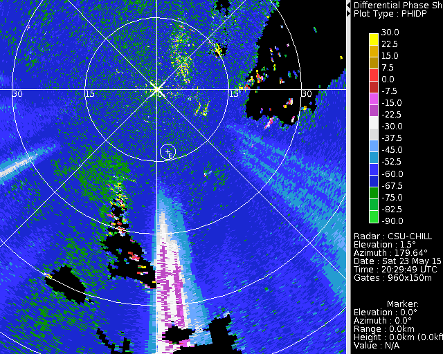
2045 UTC PPI data
The three figures below show the low elevation sweep that commenced at 2045:07 UTC. Once again, the location of the ground instrumentation site is marked with a ‘+ E’ sign, i.e. at ~ 13 km range along 171.5 deg azimuth. In this region, high Zh values are seen as well as high Zdr values, indicating the presence of large drops at and around this location around this time period. This is consistent with the DSD data shown earlier. The phidp plot shows significant differential phase shifts beyond the ground instrument site, around 45 deg which is high for S band.


DSD data and fits
The measured DSD spectra (over 3 minutes) which are used as input to the fitting procedure were constructed by utilizing the corresponding MPS-based DSD measurements for 0.15 < Deq ≤ 1 mm and the 2DVD-based DSD measurements for Deq >1 mm. Variation of the data and the fitted curves over the 90-minute period can be seen from the animation below where the MPS data are shown in black, the 2DVD data in blue and the fitted curve in red. In all cases, the fitted curves closely represent the composite DSDs, highlighting the flexibility of the model.
|
|
||
|

As an independent but qualitative verification of the ‘representativeness’ of the fitted curves, the 3 minute rainfall rates were computed from each of the fitted equations and compared with the 3 minute rain rate measurements from the collocated Pluvio. In the figure below the red line represents the estimates based on the fitted model and the purple line shows the Pluvio measurements. Shown below this plot are two examples of 3-minute DSD measurements and their corresponding fits. The left panel shows the plot for the 20:42 – 20:45 UTC period when the rainfall rate reached its maximum value of 60 mm / h, and by contrast the right panel shows the plot for 21:39 – 21:42 UTC period when the rainfall rate was below 5 mm/h. Once again, the flexibility of the fitted model is clearly evident. The model is able to capture the shape of the DSD curves for a wide range of rainfall rates. Note also that in some cases, the shapes of the DSD's resemble equilibrium DSD curves (e. g. McFarquhar, 2004).


References
Baumgardner, D., G. Kok, W. Dawson, D. O’Connor, and R. Newton, 2002: A new ground-based precipitation spectrometer: The Meteorological Particle Sensor (MPS). 11th Conf. on Cloud Physics, Ogden, UT, Amer. Meteor. Soc., 8.6. [Available online at https://ams.confex.com/ams/11AR11CP/webprogram/Paper41834.html]
Lee, G., I. Zawadzki, W. Szyrmer, D. Sempere-Torres, and R. Uijlenhoet, 2004: ‘A general approach to double-moment normalization of drop size distributions’, J. Appl. Meteor., 43, 264–281.
McFarquhar, G.M., 2004: A new representation of collision-induced breakup of raindrops and its implications for the shapes of raindrop size distributions. J. Atmos. Sci., 61, 777-794.
OTT Messtechnik GmbH, 2010: “Operating instructions Precipitation Gauge OTT Pluvio”.
Raupach, T.H. and A. Berne, 2017: Invariance of the Double-Moment Normalized Raindrop Size Distribution through 3D Spatial Displacement in Stratiform Rain. J. Appl. Meteor. Climatol., 56, 1663–1680.
Sheppard, B. E., and P. Joe, 2008: Performance of the precipitation occurrence sensor system as a precipitation gauge, Journal of Atmospheric and Oceanic Technology, Vol. 25, pp. 196-212.
Shönhuber, M., G. Lammar and W. L. Randeu, 2008: “The 2D-video-vistrometer”, Chapter 1 in “Precipitation: Advances in Measurement, Estimation and Prediction”, Michaelides, Silas. (Ed.), Springer, ISBN: 978-3-540-77654-3.
Thurai, M. P. Gatlin, V. N. Bringi, W. Petersen, P. Kennedy, B. Notaroš, and L. Carey, 2017: Toward Completing the Raindrop Size Spectrum: Case Studies Involving 2D-Video Disdrometer, Droplet Spectrometer, and Polarimetric Radar Measurements, J. Appl. Meteor. Climatol., 56 (4), 877–896.
Thurai M., and V. N. Bringi, 2017: Application of the Generalized Gamma Model to Represent the Full DSD Spectra, Extended Abstract, 38th Conference on Radar Meteorology, 5A.2, Chicago, USA. https://ams.confex.com/ams/38RADAR/meetingapp.cgi/Paper/320599